はじめに
今回 python でアニメーションを作成する方法をリサーチするにあたって気づきましたが、意外とこういう題材を扱っている記事は少ないみたいです。おそらく制御工学を本業でやっている研究者の方や学生さんは matlab を使うと思うので、python を使って運動を解析をしたりアニメーションを作ったりする人は少ないのかなと思っています。
そういう意味で、本記事やこれまで書いた記事は、趣味でロボット制御の勉強をしたい人にとって結構有益な記事なのではないかな?と自負しています。(↓前回までの記事)
立体を描画するにあたり、主に参考にしたのは以下の記事です。
これまでの記事と同様、ソースコードは github にアップしているので、ご参考にしていただければと思います。
ちなみにソースコード全体を実行すると、私の環境で 14 分弱かかります…。私の使用パソコンは dell の xps13 で CPU は intel core i7 です。
回転行列の定義
対応する節:mathematical definition of rotation matrix
$x, y, z$ 軸周りの回転行列をそれぞれ定義します。たとえば、$x$ 軸周りに $\theta$ だけ回転する行列は以下です。
\begin{align}
R_x (\theta) &= \begin{bmatrix} 1 & 0 & 0 \\
0 & \cos \theta & -\sin \theta \\
0 & \sin \theta & \cos \theta \end{bmatrix}
\end{align}
以下が対応するコードです。
def rot_x(theta):
    Rx = np.array([[1, 0, 0],
                   [0, np.cos(theta), -np.sin(theta)],
                   [0, np.sin(theta), np.cos(theta)]])
    return Rx;
物理パラメータの設定・形状の定義
対応する節:physical parameter settings and define shapes
オムニホイールロボット
オムニホイールロボットは以下のような形状として、それぞれのパラメータを定めます。
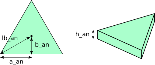
| 変数名 | 値 |
| lb_an | 0.25 |
| a_an | lb_an x 1.73 / 2 |
| b_an | lb_an / 2 |
| h_an | 0.05 |
※アニメーションを見やすくするために、シミュレーションで使っている物理パラメータとは別の値にしていることにご注意ください。
三角柱のような構造になるので、6点の座標でオムニホイールロボットは表現することができます。
def init_base_pos():
    base_pos = np.array([[lb_an, 0, 0],
                         [-b_an,  a_an, 0],
                         [-b_an, -a_an, 0],
                         [lb_an, 0, h_an],
                         [-b_an,  a_an, h_an],
                         [-b_an, -a_an, h_an]])

    return base_pos;

base_pos = init_base_pos();
さらに、オムニロボを回転させる変換と並進させる変換を定義します。
オムニロボは $z$ 軸周りに $\alpha$ 回転し、$x$ 軸と $y$ 軸方向に $x$, $y$ だけ移動するものとして、変換を表現すると以下のようになります。
base_vertex_num = 6

def rotate_base(base_pos, alpha):
    ans_pos = np.zeros((base_vertex_num, 3))
    for i in range(base_vertex_num):
        ans_pos[i] = rot_z(alpha).dot(base_pos[i])

    return ans_pos

def translate_base(base_pos, x, y):
    ans_pos = np.zeros((base_vertex_num, 3))
    for i in range(base_vertex_num):
        ans_pos[i] = [x, y, 0] + base_pos[i]

    return ans_pos
先ほど定義した base_pos 配列の要素をそれぞれ変換していきます。6つの要素(頂点)があるので、それぞれの要素に対して同じ動作をする必要があります。
振子
振子は直方体と仮定して、大きさを 2pa_an x 2pa_an x 2pl_an とします。以下のパラメータを代入すると、振子は 3cm x 3cm x 1m の直方体としてアニメーション描画をすることになります。
| 変数名 | 説明 | 値 |
| pa_an | 縦と横の長さの 1/2 の値 | 0.015 |
| pl_an | 高さの 1/2 の値 | 0.5 |
※オムニロボと同様、アニメーションを見やすくするためにシミュレーションで使っている物理パラメータとは別の値にしています。シミュレーションでは振子は 2m の長さでしたが、アニメーションでは 1m と仮定して動かしており、少しだけ動きが不自然(本来よりゆっくり)になるかと思います。
直方体なので、8つの頂点座標で表現することができます。
def init_pend_pos():
    pend_pos = np.array([[-pa_an, -pa_an, -pl_an],
                         [ pa_an, -pa_an, -pl_an],
                         [ pa_an,  pa_an, -pl_an],
                         [-pa_an,  pa_an, -pl_an],
                         [-pa_an, -pa_an, pl_an],
                         [ pa_an, -pa_an, pl_an],
                         [ pa_an,  pa_an, pl_an],
                         [-pa_an,  pa_an, pl_an]])

    return pend_pos

pend_pos = init_pend_pos()
オムニロボと同様に回転・並進を定義します。
回転に関しては、ワールド座標系の $x$ 軸周りに $\phi$ 回転させてから、回転後の座標系の $y$ 軸周りに $\theta$ 回転させる必要があるため、$R_y(\theta) R_x(\phi)$ をそれぞれの頂点の座標ベクトルにかける必要があります。
pend_vertex_num = 8

def rotate_pend(pend_pos, phi, theta):
    ans_pos = np.zeros((pend_vertex_num, 3))
    for i in range(pend_vertex_num):
        ans_pos[i] = rot_y(theta).dot(rot_x(phi).dot(pend_pos[i]))

    return ans_pos

def translate_pend(pend_pos, x, y):
    ans_pos = np.zeros((pend_vertex_num, 3))
    for i in range(pend_vertex_num):
        ans_pos[i] = [x, y, 0] + pend_pos[i]

    return ans_pos
また、振子の下端をロボットの中心と合わせる関数 adjust_pend_origin() を定義しています。
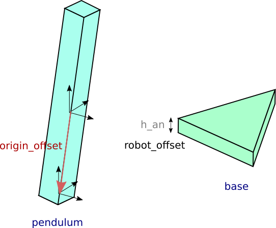
origin_offset が原点からみた振子の下端の座標に対応しており、このオフセットを打ち消すことで振子の下端を原点に持っていきます。また、robot_offset を足すことで振子の下端の $z$ 座標をオムニロボの高さに調整します。
def adjust_pend_origin(pend_pos):
    ans_pos = np.zeros((pend_vertex_num, 3))
    origin_offset = (pend_pos[0] + pend_pos[2])/2
    robot_offset  = [0, 0, h_an]
    for i in range(pend_vertex_num):
        ans_pos[i] = -origin_offset + robot_offset + pend_pos[i]

    return ans_pos
オムニロボと振子の位置・姿勢をセットする関数
対応する節:function for setting position and attitude
ここまでで定義した関数を使って、オムニロボと振子の位置・姿勢をセットする関数を定義します。以下の関数は、シミュレーションで得られた $[x, y, \alpha, \phi, \theta]^T$ の時系列データを用いて、オムニロボと振子のすべての頂点座標を適切な位置に配置する役目を担います。
def set_base_pos(base_pos, x, y, alpha):
    base_pos = init_base_pos()
    base_pos = rotate_base(base_pos, alpha)
    base_pos = translate_base(base_pos, x, y)

    return base_pos

def set_pend_pos(pend_pos, x, y, phi, theta):
    pend_pos = init_pend_pos()
    pend_pos = rotate_pend(pend_pos, phi, theta)
    pend_pos = adjust_pend_origin(pend_pos)
    pend_pos = translate_pend(pend_pos, x, y)

return pend_pos上記コードでは、「位置・姿勢の初期化 -> 回転 -> 並進移動」の流れで処理をしています。
$R_y(\theta) R_x(\phi)$ は振子の重心を基準とした回転なので、重心周りに回転させてから adjust_pend_origin() で振子の下端をロボットの中心に合わせる必要があることに注意しましょう。
3次元プロットをする関数の定義
対応する節:3dplot function
ロボットと振子を3次元プロットする関数を定義します。
def plot_pend_base(i, base_pos, pend_pos, is_save, ax_max=1.0):
    ax  = fig.add_subplot(111, projection='3d')
    base_surfs = [[base_pos[0],base_pos[1],base_pos[2]],
                  [base_pos[0],base_pos[2],base_pos[5],base_pos[3]],
                  [base_pos[0],base_pos[1],base_pos[4],base_pos[3]],
                  [base_pos[1],base_pos[2],base_pos[5],base_pos[4]],
                  [base_pos[3],base_pos[4],base_pos[5]]]
    ax.add_collection3d(Poly3DCollection(base_surfs, facecolors='green', linewidths=0.5, edgecolors='white', alpha=0.9))

    pend_surfs = [[pend_pos[0],pend_pos[1],pend_pos[2],pend_pos[3]],
                  [pend_pos[0],pend_pos[3],pend_pos[7],pend_pos[4]],
                  [pend_pos[1],pend_pos[2],pend_pos[6],pend_pos[5]],
                  [pend_pos[4],pend_pos[5],pend_pos[6],pend_pos[7]],
                  [pend_pos[0],pend_pos[1],pend_pos[5],pend_pos[4]],
                  [pend_pos[3],pend_pos[2],pend_pos[6],pend_pos[7]]]
    ax.add_collection3d(Poly3DCollection(pend_surfs, facecolors='blue', linewidths=0.5, edgecolors='white', alpha=0.9))

    ax.set_xticks([-ax_max, -ax_max/2, 0.0, ax_max/2, ax_max])
    ax.set_yticks([-ax_max, -ax_max/2, 0.0, ax_max/2, ax_max])
    ax.set_zticks([0.0, ax_max/2, ax_max])
    ax.set_xlabel("x", size = 20)
    ax.set_ylabel("y", size = 20)
    ax.set_zlabel("z", size = 20)

    if is_save == True:
        plt.savefig('pictures/animation/image/img_' + str(i) + '.png')
    else:
        plt.show()
パッと見複雑ですが、やっていることは以下の通りです。
- 頂点同士を結んで平面を定義する
たとえば [base_pos[0],base_pos[2],base_pos[5],base_pos[3]] は、base_pos の 4 点の座標から構成される平面となります。 - これらを並べた配列 base_surfs, pend_surfs を作る
- add_collection3d() という関数でこれらを描画する
色や透過率、線の設定も変更することができます。 - 引数 is_save が True のときは、指定したパスに画像を保存する
保存した画像は後のアニメーション描画で使います。
※指定したディレクトリがないとエラーするので、ディレクトリを予め作っておく必要があります。
軸ラベルの設定方法等についてはこのサイトを参考にしました。ax_max のデフォルト値は 1.0 としています。
3次元プロットのテスト
対応する節:test 3d plot
3次元プロットのテストをここで行います。数値例を入力して、base_pos, pend_pos を定め、これらを先に定義した関数 plot_pend_base() に代入して3次元プロットしています。
base_pos = set_base_pos(base_pos, x_pos_an, y_pos_an, alpha_an)
pend_pos = set_pend_pos(pend_pos, x_pos_an, y_pos_an, phi_an, theta_an)

fig = plt.figure(figsize=(10.0, 10.0))
plot_pend_base(0, base_pos, pend_pos, True)
たとえば、$[x, y, \alpha, \phi, \theta]^T = [0.3, -0.3, 0.2, 0.0, 0.2]^T$ と設定して描画を試してみた結果、以下のような図が得られます。
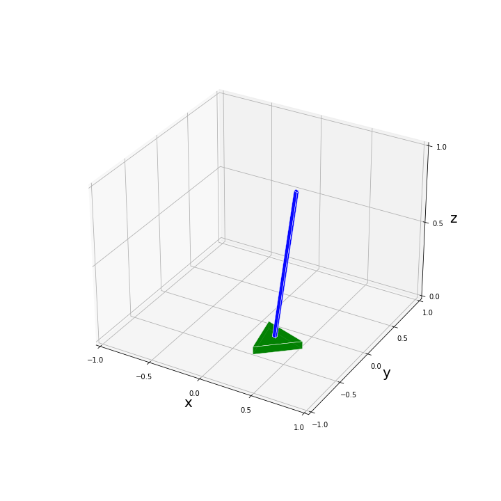
$x, y, \alpha$ の回転・並進移動に関してはパッと見てすぐに問題なく反映されていることがわかると思います。振子の傾きが合っているかを上図から判定するのは難しいですが、いくつか数値を代入してみて問題なく描画されていることを確認しました。
アニメーション用のシミュレーションデータ作成
対応する節:create simulation data for animation
アニメーション描画のために画像を保存しますが、保存する枚数が多いとかなり時間がかかってしまうので、短めのシミュレーション時間 & すこし長めのシミュレーション間隔に設定してデータを作成しました。
※このとき、シミュレーション間隔をいたずらに長くしてしまうと計算結果が現実と乖離しシステムが不安定化してしまったため、間隔は大きくしすぎないようにしました。
シミュレーション時間を 5s、間隔を 0.05s としました。このとき、保存される画像は 100 枚になります。
初期状態は以下のように設定しました。
\begin{align}
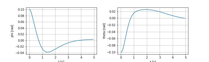
[x_0, y_0, \alpha_0, \phi_0, \theta_0, \dot x_0, \dot y_0, \dot \alpha_0, \dot \phi_0, \dot \theta_0]^T &= [0, 0, 0, 0.1, -0.1, 0, 0, 0, 0, 0]^T \\
[u_{1, 0}, u_{2, 0}, u_{3, 0}]^T &= [0, 0, 0]^T
\end{align}
つまり、初期状態は $[\phi, \theta]^T = [0.1, -0.1]^T$ で、それ以外は 0 としています。0.1 rad は約 5.73 deg です。
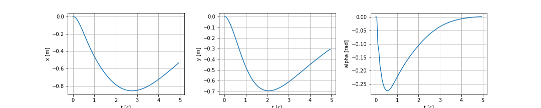
シミュレーションの実行とグラフの描画は、以下コマンドで行っています。
[t_sim, x_sim, u_sim] = execute_simulation(T_sim, dt_sim, x0_sim, u0_sim)
plot_x_y_alpha(t_sim, x_sim)
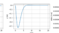
plot_phi_theta(t_sim, x_sim)シミュレーション結果のグラフを見てみると、5 s 間でも安定化できていそうです。
アニメーション用画像データの生成
対応する節:create images for animation
$[x, y, \alpha, \phi, \theta]^T$ の値を、作成したシミュレーションの時系列データから抽出して3次元プロットを行い、出来上がった画像をフレームごとに保存していきます。
def create_animation_images(t_sim, x_sim, base_pos, pend_pos, ax_max=1.0):
    for i in range(len(t_sim)):
        x_pos_an = x_sim[i, 0]
        y_pos_an = x_sim[i, 1]
        alpha_an = x_sim[i, 2]
        phi_an   = x_sim[i, 3]
        theta_an = x_sim[i, 4]

        base_pos = set_base_pos(base_pos, x_pos_an, y_pos_an, alpha_an)
        pend_pos = set_pend_pos(pend_pos, x_pos_an, y_pos_an, phi_an, theta_an)
        plot_pend_base(i, base_pos, pend_pos, True, ax_max)

fig = plt.figure(figsize=(10.0, 10.0))
create_animation_images(t_sim, x_sim, base_pos, pend_pos)
gif 形式でのアニメーションのファイル保存と描画
対応する節:save as a gif file and display
指定したパス(’pictures/animation/image/’)からファイル名が img_数字.png となっている画像を image 配列に順番に格納し、最後にこれを指定された filename の gif ファイルに保存します。(参考サイト)fps はシミュレーション間隔の逆数なので、1/dt_sim を代入します。
また、Image(filename=filename_gif, width=800) で jupyter notebook 上に gif ファイルの描画をします。
def save_images_as_gif(dt_sim, t_sim, filename):
    images = []
    for i in range(len(t_sim)):
        images.append(imageio.imread('pictures/animation/image/img_' + str(i) + '.png'))

    imageio.mimsave(filename, images, fps=1/dt_sim)

filename_gif = 'pictures/animation/test1.gif'
save_images_as_gif(dt_sim, t_sim, filename_gif)
Image(filename=filename_gif, width=800)
描画されたアニメーションから、システムは初期状態 $[\phi, \theta]^T = [0.1, -0.1]^T$ から安定化可能であることがわかります。
初期状態を変えた場合のシミュレーション
対応する節:other simulations
$\phi$ と $\theta$ が大きい値の場合
$[\phi, \theta]^T = [0.25, -0.25]^T$ を初期状態(その他はすべて 0)としたときのシステムの挙動をアニメーションで確認してみます。ちなみに 0.25 rad は約 14.3 deg です。
アニメーションから、一応システムは安定化可能であることがわかりました。$x, y$ 軸両方に 2 m 以上移動するので、$x, y$ の表示範囲を $\pm 2$ m 、$z$ の表示範囲を 0 – 2 m としています。
現実のシステムだとノイズや遅れが入るため、このレベルの初期角度がついているとおそらく安定化は困難な気がしますね…。また、モータの最大出力の関係でこのレベルの入力 $u$ を実現できない可能性もあるため、モデル予測制御等の制約を考慮した制御則を適用する必要もあるかもしれません。
$\alpha$ が非ゼロの場合
$[\alpha, \phi, \theta]^T = [1.57, 0.1, -0.1]^T$ を初期状態(その他はすべて 0)としたときのシステムの挙動をアニメーションで確認してみます。ちなみに 1.57 rad は約 90 deg です。
こちらも少しアグレッシブな挙動にはなりますが、問題なく安定化できています。動き面白いですね。
$x, y$ が非ゼロの場合
$[x, y, \phi, \theta]^T = [-0.5, 0.5, 0.1, -0.1]^T$ を初期状態(その他はすべて 0)としたときのシステムの挙動をアニメーションで確認してみます。
この場合もシステムは安定化できていますね。
結論、今回試したすべての初期状態で、システムの安定化は達成されました。
まとめ
本記事では python でアニメーションを作成する方法を解説しました。
今回は LQR 制御則を適用していますが、モデル予測制御等を適用してどのようにふるまいが変わるかをチェックしていくのもおもしろいかもと思いました。あとは、実機の製作もできればやってみたいと思っています。

コメント